X-Ray Imaging
Conventional radiographic imaging of the petrous portion of the temporal bone and mastoid was historically one of the primary methods for examining ear diseases but has now largely been replaced by temporal bone CT scans. Currently, the modified Stenver’s view, also known as the cochlear view, remains in use. This method primarily aims to visualize the position of the cochlear implant in the temporal region and the placement of the electrodes within the cochlea.
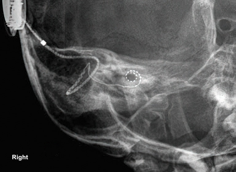
Figure 1 X-ray image in cochlear view
CT Scanning
CT scanning of the ear provides detailed imaging of the delicate anatomical structures of the temporal bone, including the external auditory canal, the three ossicles, the facial nerve canal, the internal auditory canal, the sigmoid sinus, the openings of the vestibular aqueduct and cochlear aqueduct, the cochlea, the vestibule, and the three semicircular canals. Besides offering high-resolution visualization of the intricate bony structures of the temporal bone, CT scanning can also reveal abnormal soft-tissue shadows. This technique holds significant diagnostic value in assessing congenital ear deformities, temporal bone fractures, various middle ear infections, and tumors.
Routine ear CT scans involve coronal and axial (horizontal or transverse) planes with a slice thickness of 2 mm. Coronal images typically focus on three key planes: the cochlea, the vestibule, and the mastoid. In the coronal plane, slices are oriented perpendicular to the auditory brow line (a line connecting the external auditory canal opening to the ipsilateral supraorbital rim) and are scanned layer by layer from anterior to posterior, starting at the anterior edge of the external auditory canal. Coronal images, particularly when bone scans of individual sides are magnified, provide clear views of the middle ear structures.
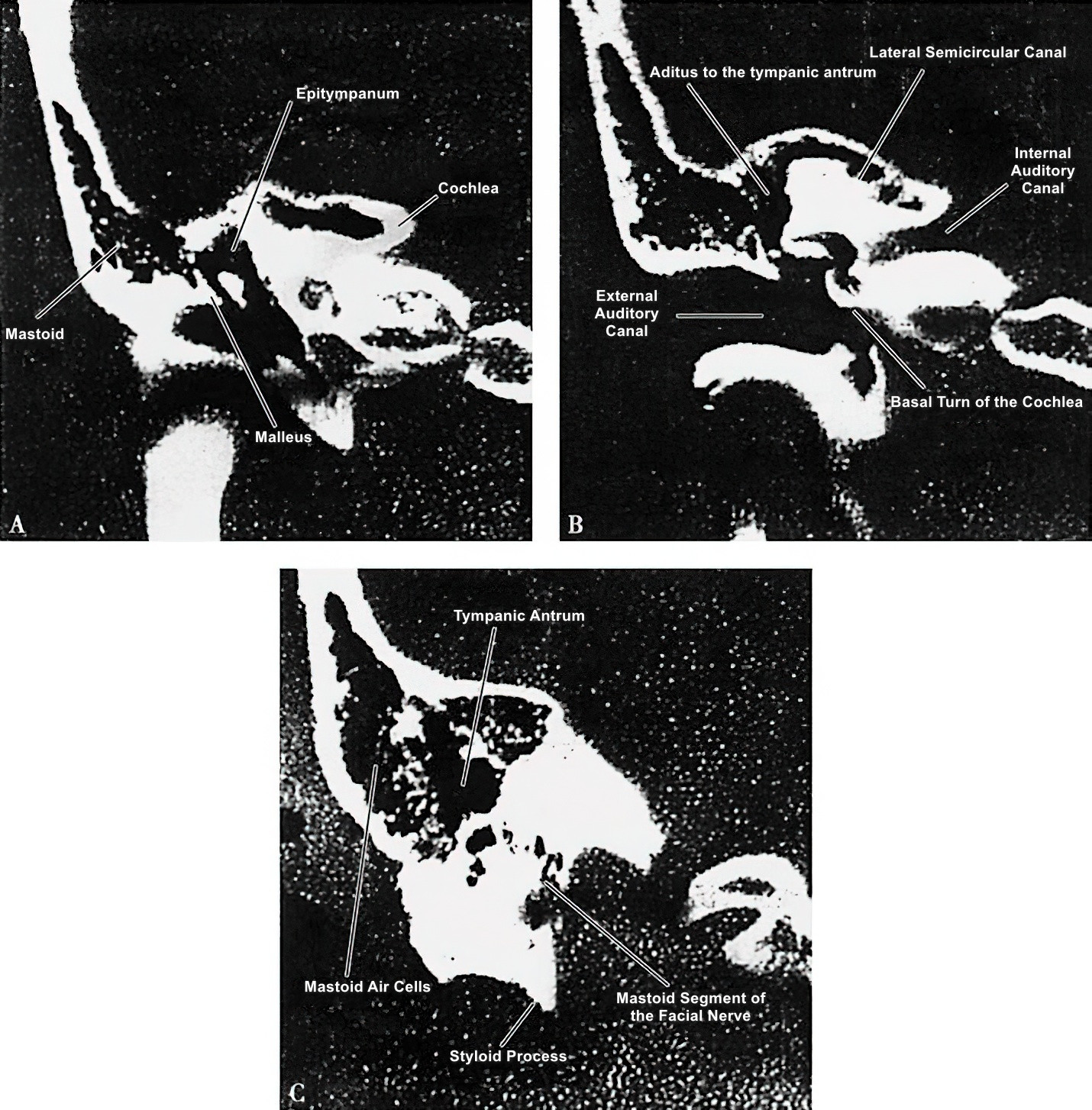
Figure 2 Coronal CT scan of the temporal bone
A. Coronal CT scan showing the cochlear plane of the temporal bone.
B. Coronal CT scan showing the vestibular plane of the temporal bone.
C. Coronal CT scan showing the mastoid plane of the temporal bone.
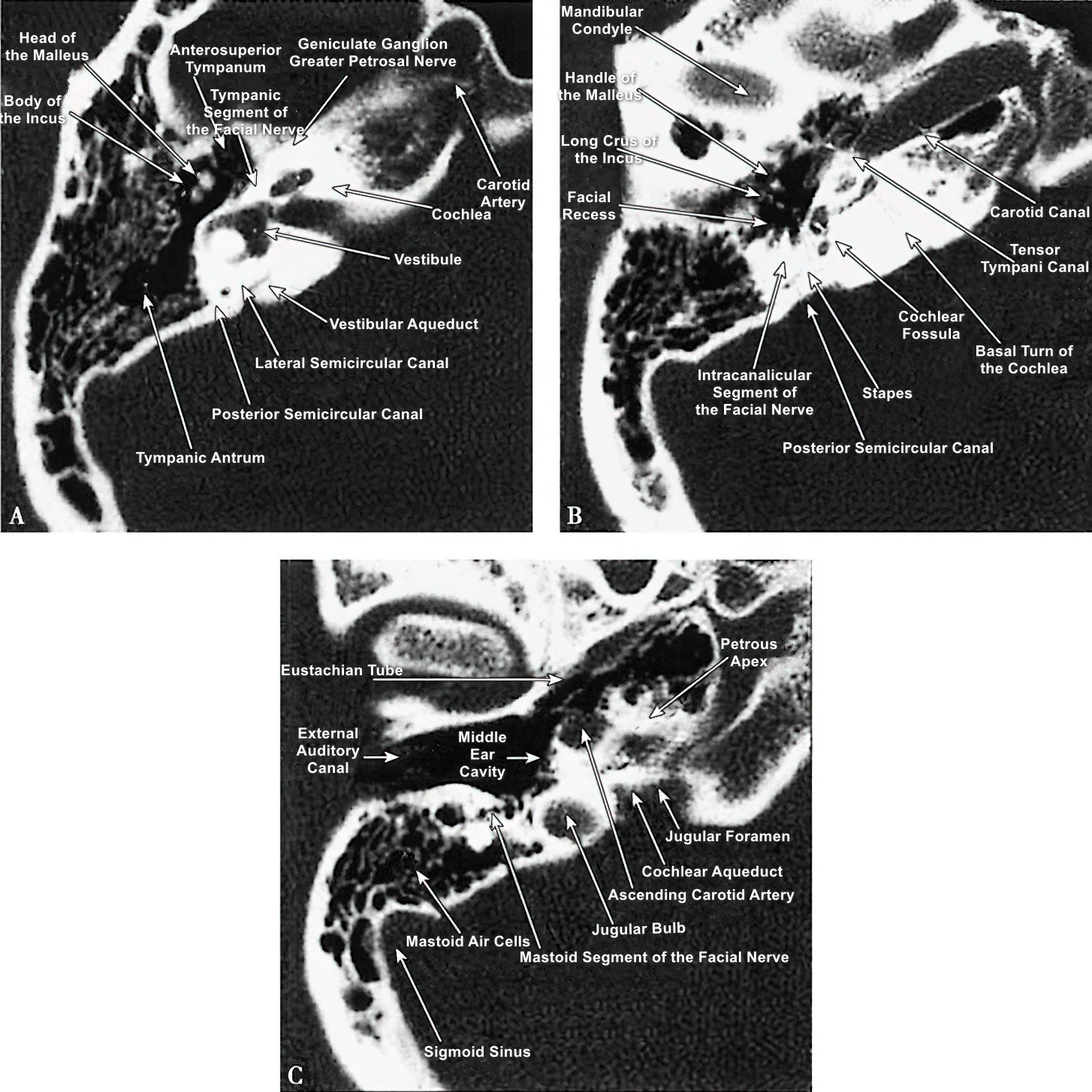
Figure 3 Axial CT scan of the temporal bone
A. Axial CT scan showing the vestibular plane.
B. Axial CT scan showing the cochlear plane.
C. Axial CT scan showing the mastoid plane.
Axial images use the line connecting the upper edge of the external auditory canal to the highest point of the supraorbital rim as the baseline and are scanned layer by layer from inferior to superior. These scans clearly depict the inner ear and internal auditory canal. The combination of coronal and axial CT images offers valuable data that conventional X-rays cannot provide, aiding in the diagnosis of ear diseases and preoperative evaluation.
MRI
Magnetic resonance imaging (MRI) provides detailed visualization of the soft tissue structures of the inner ear and internal auditory canal. MRI is particularly useful for displaying the changes in soft tissue structures of the cerebellopontine angle, temporal lobe, and ventricles associated with temporal bone lesions, such as tumors, abscesses, and hemorrhages.
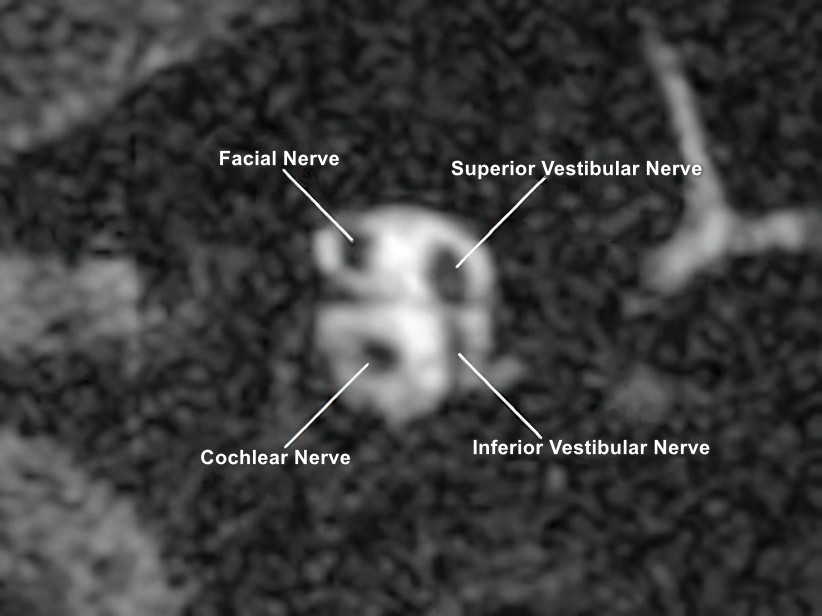
Figure 4 MRI of the internal auditory canal
Inner Ear Imaging via MRI
Although the perilymph and endolymph are not directly connected and differ in ionic composition, the Reissner's membrane is too thin to be detected by standard MRI techniques. As a result, conventional MRI and MR water imaging are unable to delineate the boundary between the perilymphatic and endolymphatic spaces, limiting visualization of the endolymph. Gadolinium-enhanced imaging is currently the main method for visualizing inner ear fluids, with two contrast delivery approaches available: transtympanic (via the middle ear) and intravenous administration.
Transtympanic Gadolinium Administration
In this approach, gadolinium contrast medium is diluted with saline in a 1:7 ratio. Approximately 1–2 mL of this solution is then injected into the middle ear cavity through a tympanic membrane puncture. After transtympanic injection, the gadolinium penetrates the round window membrane or enters the perilymphatic fluid via the annular ligament perilymphatic space, while the endolymph remains contrast-free. About 24 hours post-injection, the concentration of the contrast agent peaks in the perilymph, significantly enhancing the imaging contrast between the perilymph and endolymph spaces, allowing the membranous labyrinth morphology to be visualized.
Intravenous Gadolinium Administration
With this method, gadolinium contrast is not diluted and is injected intravenously at a dosage of 0.2 mmol/kg. Approximately four hours post-injection, the concentration of the contrast agent in the perilymph reaches its peak. MRI scanning at this point reveals the morphology of the membranous labyrinth. The technique avoids the need for direct middle ear injections but has the limitation of providing images with lower clarity compared to transtympanic injection.
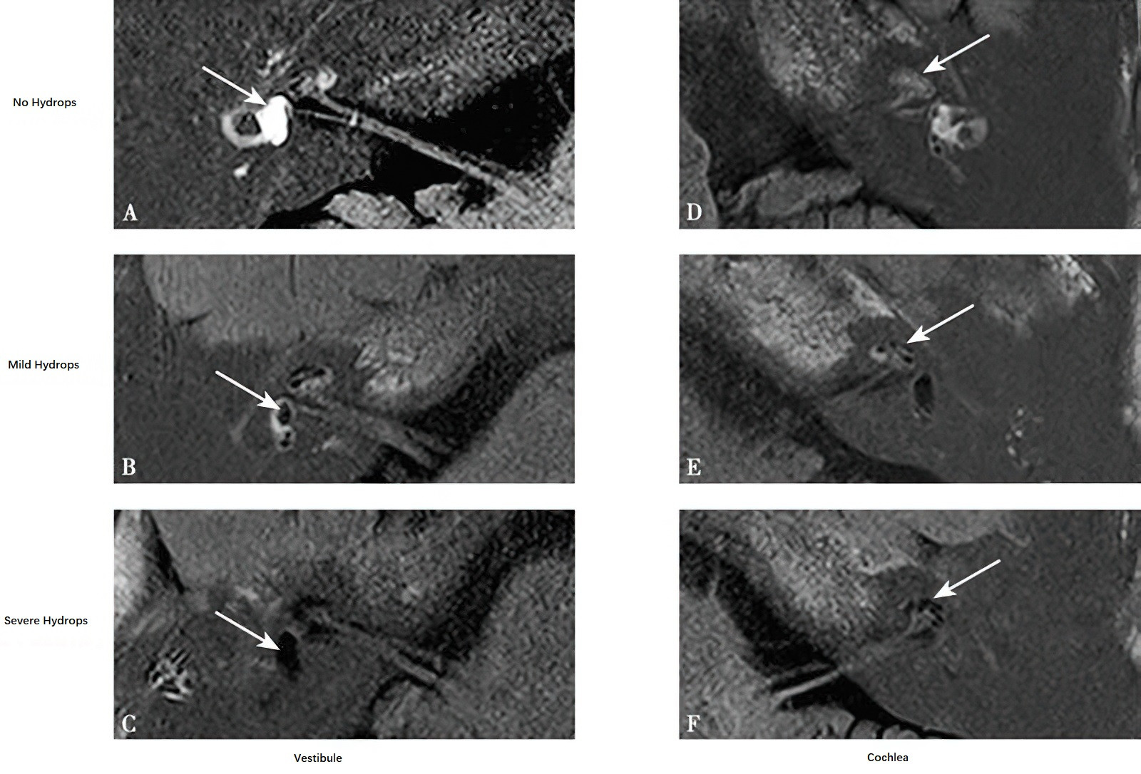
Figure 5 Inner ear MR imaging with gadolinium contrast
A, D. Normal Endolymph.
B, C, E, F. Endolymphatic Hydrops.